Simulations
For the simulation of our system the software that was been used is Homer Pro. Homer Pro is an optimization tool that based on technical feasibility and cost criteria determines the optimal number of components for the modeled system
Electrical and Hydrogen Production
The results of the simulations showed that to satisfy our hydrogen demand of 644.58 kg/h for the ferries and the electricity demand for the liquefaction process of the hydrogen, 7735 kW/h, we need the number of components shown in Table 1. Moreover the storage has been selected manually in order to have a five day demand of hydrogen as backup for large periods with no electricity production. The production of electricity and the production of hydrogen for each month are given in Figure 1. The total electricity production for a year is 487.09 GWh and the total hydrogen production is 5718.55 tonnes.
Table 1 : Components of the modeled system
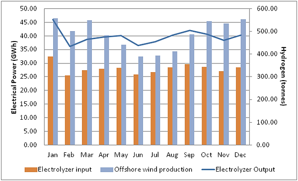
Figure 1: Electrical and hydrogen production per month
As it can be observed in Figure 1, the production of electricity from the offshore wind farm is significantly more that the demand needed for the electrolyzer in each month. The results showed that this excess energy with the satisfaction of the electric load is 16.9 % of the total energy production in a year. This excess energy creates the opportunity of having another cash flow something that we examine in the financial analysis. In addition the month of January has the biggest production of hydrogen because it was assumed in the simulations that at the beginning of the year the storage was empty. The reasoning behind this is explained in the section bellow
System Operation
Knowing the stochastic nature of wind farms is essential to see how the system works when there is no production of electricity from the wind farm. Two cases for the operation of the system were examined:
Start of the Year
In Figure 2 and Figure 3 a snapshot of the system is given for the hydrogen production and the electricity production respectively at the beginning of the year. This time period was chosen in order to illustrate how our system works in the worst case scenario were the storage is empty.
In Figure 2 is showning that the system is overproducing when the offshore wind farm is producing in full capacity in order to insure that the demand is reached when there is no electricity production. Moreover, at those time periods an increasing trend of the level of the storage. The data have shown that the system needs 11 days to reach the full capacity storage and after that is kept relatively full with some fluctuations. In addition when the system is overproducing the excess electricity is minimum. Finally the batteries are connected to the system to cover the need of electricity for the liquefaction process.
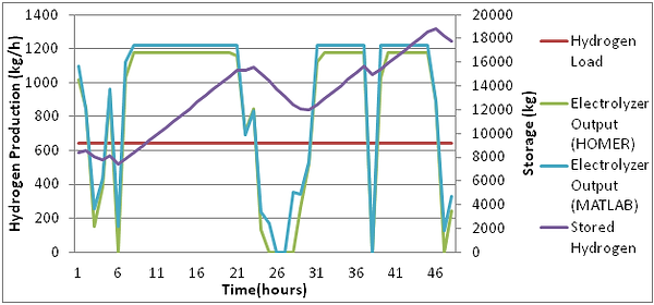
Figure 2: Hydrogen production of the system for 48 hours at the beginning of the year.
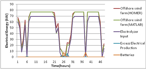
Figure 3: Electrical production of the system for 48 hours at the beginning of the year.
Middle of the year
In Figure 4 and Figure 5 a snapshot of the system is given for the hydrogen production and the electricity production respectively at the middle of the year. This time period was chosen in order to illustrate how our system works when the storage is full. As shown in Figure 4 when the storage is full the production of hydrogen is limited to the demand per hour and as a result the excess energy in Figure 5 is significantly more than the one observed in Figure 3.

Figure 4: Hydrogen production of the system for 48 hours at the middle of the year.

Figure 5: Electrical production of the system for 48 hours at the middle of the year.
Verification of the results
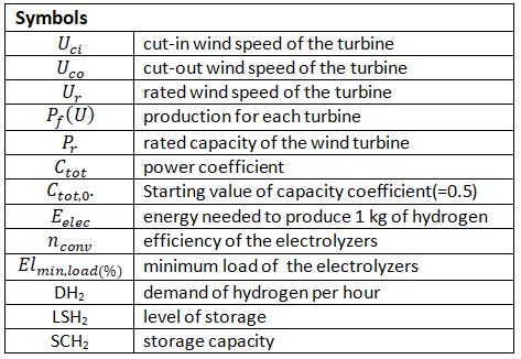
To verify the results from Homer a modeled on Matlab was created using the equations 1-5 which were taken from [1]. For the offshore wind farm output , 4 different scenarios were identified as shown in eq. 2. Firstly when the wind speed is below the cut-in speed or when the wind speed is over the cut-off wind speed, there is no production of electricity. Secondly when the wind speed is between the cut-in speed and rated wind speed of the turbine, the production for each turbine is calculated using eq. 1.Finally when the wind speed is between the rated wind speed and the cut-off speed the wind turbine is producing at its rated capacity. The total electrical output of the wind farm is calculated using eq.3.


The production of hydrogen is calculated using eq.5. Like the electricity production for the production of hydrogen there are 4 different scenarios shown in eq.6. The main factor in these scenarios is the level of the storage of hydrogen .Firstly when the output of the wind farm is below the minimum load of the electrolyzers there is no production of hydrogen. Secondly when the storage has room for any excess hydrogen beyond the demand of hydrogen per hour the production of hydrogen is limited. Thirdly when the storage is in full capacity the production is limited to the demand of hydrogen per hour .Lastly the production is limited when the production of hydrogen is more than the demand and there is not enough space in the storage tank.

References
[1] Van Nguyen Dinh, Paul Leahy, Eamon McKeogh, Jimmy Murphy, Val Cummins,Development of a viability assessment model for hydrogen production from dedicated offshore wind farms, International Journal of Hydrogen Energy,2020,ISSN 0360-3199,https://doi.org/10.1016/j.ijhydene.2020.04.232.
Homer Pro simulation values and matlab code